Linear Regression and DC Power Flow

Linear Regression and DC Power Flow

In class we learned that the DC approximation of the power flow problem linearizes the relationship between the phase angle and power injections over a power grid, like the example in Fig. 1. In this notebook we’ll use linear regression with L1 (LASSO) and L2 (ridge) regularization to estimate the phase angle, line characteristics, power injections, flows, under various conditions.

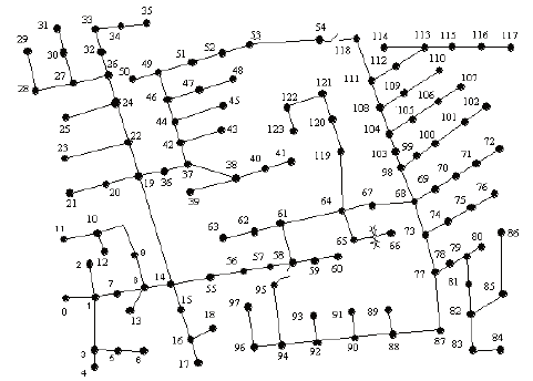
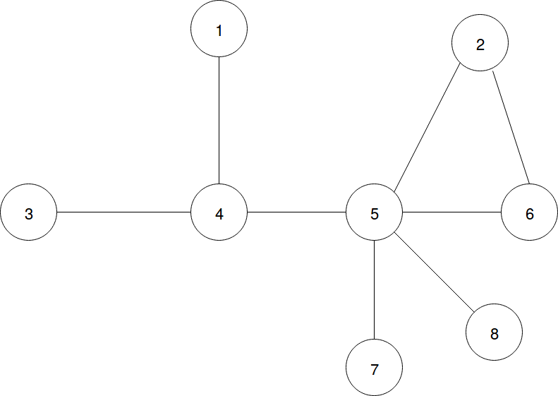
First we’ll need to go over a few definitions and matrices that you saw in class. Fig. 1 illustrates the IEEE-123 test feeder, a standardized distribution network used to test control algorithms and optimization techniques for application in real systems. Each node in the graph is an electrical bus, and each edge is a power line. In the programming assignment questions, we’ll be looking at a much simpler, 8-bus network we design ourselves. Note that each bus has a number assigned to it.

In AC (DC) power flow, electricity is subject to impedance (resistance) over the power lines. We can represent this with a special $n x n$ matrix which characterizes this impedance at each node and between nodes. Based on how the power flow problem is simplified, the values of these matrix are called admittance or susceptance because these values become inverted, or only represent a real or imaginary part of the power flow. Regardless, the structure remains the same; we’ll define the admittance matrix, $B$, as

If two nodes $i,j$ are connected, the line has admittance $b_{i,j}$. The diagonal elements are the sum of the admittances of the lines connected to that node. The important takeaway is that the matrix $B$ characterizes the resistivity properties of the power lines and the power line topology.

For a network, or graph like the example in Fig. 1 with $n$ nodes and $m$ edges, the node-edge incidence matrix is an $n x m$ matrix $F$ where each element is 1 if node $i$ is connection to node $j$, $-1$ if $j$ is connected to $i$ (we assign a direction), and 0 if no connection exists.

In our application we’ll scale these 1’s a 0’s by the admittance $b$, so that,

In power engineering often time we’ll assume a nominal voltage of 1 so that the power flow between busses is entirely characterized the by the AC phase angle difference between busses. If the phase angle differences are small, we can use the small angle approximation to linearize the AC power flow equations. This is called the DC approximation as it resembles the equations for DC power flow. For a vector of bus voltage angles $\boldsymbol{\theta}$ and unit voltage, then the power injection at each node,

and the power flow $\boldsymbol{f}$ along each line equals,

These are just linear equations, like we’ve seen in the previous homeworks. Moreover, phase angles are very difficult to measure, and we often work with many noisy samples of power injections and flows. For convenience, we can stack the two linear equation in a single equation:

In the following exercises we’ll look at estimating the phase-angle state of the grid.

The linear system $z = Hx$ is overdetermined. In order to find a unique solution that satisfies various operational constraints, there are tricks and techniques that power engineers use, like incorporating a so-called slack bus, or using the Kron reduction, to determine values that the engineer cares about. We’ll use what we’ve learned thus far: we can write this overdetermined system as,

where r is some residual error between a phase angle vector $x$ and the power flows and injections $z$. If we wrap the left hand side up in a 2-norm,

minimizing the residual $r$ is just like the least squares problem. In the following problems we’ll solve for the power injections and line flows using least squares, and examine the effect bad data has on our solution, and how we can adapt to it.

#here we'll construct the neccessary matrices for the above example network

import numpy as np
import matplotlib.pyplot as plt

#node edge incidence matrix scaled by admittance
#these are just arbitrary admittance values for this assignment
F = np.array([[5.0,0.0,0.0,-5.0,0.0,0.0,0.0,0.0],
              [0.0,3.0,0.0,0.0,-3.0,0.0,0.0,0.0],
              [0.0,3.0,0.0,0.0,0.0,-3.0,0.0,0.0],
              [0.0,0.0,13.0,-13.0,0.0,0.0,0.0,0.0],
              [0.0,0.0,0.0,10.0,-10.0,0.0,0.0,0.0],
              [0.0,0.0,0.0,0.0,5.0,-5.0,0.0,0.0],
              [0.0,0.0,0.0,0.0,3.2,0.0,-3.2,0.0],
              [0.0,0.0,0.0,0.0,2.5,0.0,0.0,-2.5]])

self_admittance = np.sum(np.abs(F), axis=0)

off_diag = np.array([[0, 0, 0, -5, 0, 0, 0, 0],
                     [0, 0, 0, 0, -3, -3, 0, 0],
                     [0, 0, 0, -13, 0, 0, 0, 0],
                     [-5, 0, -13, 0, -10, 0, 0, 0],
                     [0, -3, 0, -10, 0, -5, -3.2, -2.5],
                     [0, -3, 0, 0, -5, 0, 0, 0],
                     [0, 0, 0, 0, -3.2, 0, 0, 0],
                     [0, 0, 0, 0, -2.5, 0, 0, 0]])

#admittance matrix
B = np.diag(self_admittance) + off_diag

#stacked
H = np.vstack((F, B))

#true flows and power injections for reference

f = 0.01*np.array([-1, -2, -1, 20, 17, 1, 10, 3])
p = 0.01*np.array([-1, -3, 20, -2, 0, -1, -10, -3])

z = np.expand_dims(np.append(f, p), axis=1)

#to simplify our code, we can now use the least squares method in sklearn
#https://scikit-learn.org/stable/modules/generated/sklearn.linear_model.LinearRegression.html
from sklearn import linear_model

#here's an example of how to use least squares to find the lowest energy solution to an 
#overdetermined linear system, in this case we have a _single_ sample of z

model = linear_model.LinearRegression().fit(H, z)

#notice that the object model isn't the vector x
print("Output of linear_model.LinearRegression().fit() method")
print(model)
print("\n")

#it's an object with a large number of attributes, we can inspect them with the native Python function dir():
print("Attributes of model object")
print(dir(model))
print("\n")

Output of linear_model.LinearRegression().fit() method
LinearRegression(copy_X=True, fit_intercept=True, n_jobs=1, normalize=False)


Attributes of model object
['__abstractmethods__', '__class__', '__delattr__', '__dict__', '__dir__', '__doc__', '__eq__', '__format__', '__ge__', '__getattribute__', '__getstate__', '__gt__', '__hash__', '__init__', '__init_subclass__', '__le__', '__lt__', '__module__', '__ne__', '__new__', '__reduce__', '__reduce_ex__', '__repr__', '__setattr__', '__setstate__', '__sizeof__', '__str__', '__subclasshook__', '__weakref__', '_abc_cache', '_abc_negative_cache', '_abc_negative_cache_version', '_abc_registry', '_decision_function', '_estimator_type', '_get_param_names', '_preprocess_data', '_residues', '_set_intercept', 'coef_', 'copy_X', 'fit', 'fit_intercept', 'get_params', 'intercept_', 'n_jobs', 'normalize', 'predict', 'rank_', 'score', 'set_params', 'singular_']

#notice that the "Methods" section of the LinearRegression manual page linked above lists 
#several attributes that appear in the list we printed with dir(). We care about 'coef_', this is the vector x
print("Solution")
print(model.coef_)
print("\n")

#we can set this value to a variable and look at the error
x_hat = model.coef_.T  #transpose it from (1,8) to (8,1)
loss = np.linalg.norm(H.dot(x_hat) - z, 2)

print("Error")
print(loss)
print("\n")

Solution
[[ 0.01365549 -0.00781091  0.03103551  0.01564802 -0.00130978 -0.00461427
  -0.03288193 -0.01372213]]


Error
0.007751846059803475

Problem 1

For this problem you’ll need to read the manual page of the linked in the above example carefully. You’re given $k$ noisy samples of $z$: the line flows and power injections. Instantiate a linear model and find the solution $x$ of nodal phase angles. Print the loss (1 value across all samples). Hint: you’re going to find an $x$ for each sample of $z$, we need to find the best $x$ the minimizes the loss for any $z$.

#here are the samples, they are not formatted correctly, you'll need to format them correctly 
#in order to use linear_model.LinearRegression().fit()
samples_1 = []

for i in range(2):
    samples_1.append(z + np.random.normal(0,0.02,size=z.shape)) #the true value + some noise

#insert your code here

Problem 2

Our example power grid has very good power injection sensors with very little noise variance, and our cheaper line flow sensors have very high noise variance. In the example below, we show how to performed weighted least squares, in order to bias the solution to rely on the high quality data more than the low quality data.

weights = np.ones(z.shape)[:,0]  #the weights object must be 1-dimensional
model = linear_model.LinearRegression().fit(H, z, sample_weight=weights)  
x_hat = model.coef_.T

#here I've just passed in weights equal to 1, so the solution is unchanged

Find a vector of sample weights that improves on the loss over the vector of weights all equal to 1.

samples_2 = []

for i in range(100):
    injection_noise = np.random.normal(0,0.01,size=z[0:8].shape)  #variance equal to 0.01
    line_noise = np.random.normal(0,0.03,size=z[0:8].shape)       #variance equal to 0.03
    samples_2.append(z + np.expand_dims(np.append(line_noise,injection_noise),axis=1)) #the true value + some noise

#insert your code here

Problem 3

We are again given a sequence of observations of power flows and injection, but there are several bad measurements. The noise is Gaussian; use what we know about the Gaussian distribution to derive a threshold-type means of eliminating outlier data. Compare the loss of the model with and without the outliers.

#16 x 100 array of z samples
samples_3_array = np.loadtxt("homework_3_data.txt")

#insert your code here