Practical Classification: Logistic Regression

Practical Classification: Logistic Regression

Classification is an important task in data science: given some data Two common classification algorithms are logistic regression and support vector machines (SVMs), but there are many algorithms to choose from. In this homework we’ll focus on logistic regression and walk through some practical examples of binary classification: where data can either be one of two classes, which we label 0 or 1. Ultimately, classifiers like logistic regression and SVM, which we’ll talk about in the next assignment, try to find a line that seperates the input data on one of two sides.

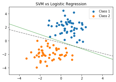
Fig. 1 illustrates the primary intuition behind a classifier. Each point represents data from some measurements. The blue class and the orange class each represent something about that data: for example, the measurements were from people testing positive or negative for a virus. A classifier finds a line that seperates the data according to the training data we use, which is very nicely seperated in this example (it almost never is in reality). SVM and Logistic regression come up with slightly different decisions boundaries, illustrated in the figure. We’ll talk about the differences in the next assignment.

Fig. 1: SVM (dashed) and Logistic Regression (solid) decision boundaries

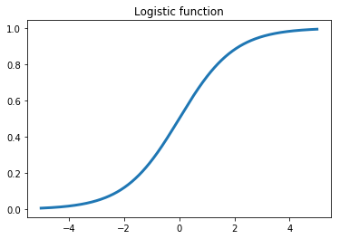
The logistic loss function is derived from the logistic function. What’s important to notice is that the output switches between 0 and 1—gradually—based on the input value. This is a critical ingredient for neural networks which we’ll get to make use of in future assignments and partly why it’s called a neural network. Biological neurons switch from outputing no signal to outputting a full signal once they’ve recieved a sufficient signal from input neurons, with some noisy-ness due in part to the chemical process that governs the input and output interactions. The probability that a neuron will fire looks a lot like a logistic function.

Fig. 2: Outputing 0 or 1

import numpy as np
import matplotlib.pyplot as plt
import sklearn.metrics
from sklearn.svm import SVC
from sklearn.linear_model import LogisticRegression

We’ve seen in previous assignments how to use sklearn’s built in data analysis tools. Using these classification algorithms is very similar, so I won’t be providing example code. I’ve imported the appropriate libraries above. Read the manpage for Logistic Regression and before starting the assignment to see example usage and what each input value is for. Just like the previous assignments we declare a model object, then use the .fit() method.

You will also need to compute the precision and recall of your classifiers. Refer to this really good Wikipedia article on the difference. Either write your own functions, or use sklearn’s built-in precision and recall functions in the sklearn.metrics library I’ve imported for you above.

#data for assignment
training_data = np.loadtxt("homework_5_train.txt")
X_train = training_data[:,0:2] #selects columns 1 and 2, which are the x and y coords of the data
Y_train = training_data[:,2] #selections column 3, which is the 0 or 1 label of the data

test_data = np.loadtxt("homework_5_test.txt")
X_test = test_data[:,0:2]
Y_test = test_data[:,2]

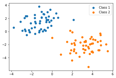
#plotting each class seperately, not important for training the models
X_1 = []
X_2 = []
for row in range(X_train.shape[0]):
    if Y_train[row] == 0:
        X_1.append(X_train[row,:])
    else:
        X_2.append(X_train[row,:])
X_1 = np.asarray(X_1)
X_2 = np.asarray(X_2)

plt.scatter(X_1[:,0], X_1[:,1], label="Class 1")
plt.scatter(X_2[:,0], X_2[:,1], label="Class 2")
plt.legend()
plt.show()

Problem 1

Use logistic regression on the training data set X_train and Y_train, train a classifier. Compute and print the training precision and recall.

#insert your code here

logreg_model_obj = LogisticRegression()

Problem 2

Using the classifier trained in problem 1, compute the precision and recall of the model on the testing data set X_test and Y_test.

#insert your code here

Problem 3

The the noise in our data is Gaussian; compare the empirical mean and variance of the training and test data sets (remember, each row of the train and test sets are a 2-dimensional sample, so the empirical mean and variance are 2 dimensional). In your own words, why might the test performance be lower?

#insert your code here

Bonus 1

Create two scatter plots: one plot for the training data as above, and one for the test data. Use sklearn’s model_object.decision_function() method to draw the decision boundaries of each model. A tutorial can be found here for plotting an SVM’s decision function, which we’ll be getting into next week. The procedure for drawing the decision boundary is identical for the logistic regression model.

#insert your code here