Practical Classification: Support Vector Machines

Practical Classification: Support Vector Machines

Like logistic regression, Support Vector Machines (SVM) are are another commonly used algorithm for classification. The primary difference between these algorithms is their loss functions, in the binary case:

SVM loss: $\mathcal{L}(y, \hat{y}) = \sum_{i} y_i - \max(0, 1 - y_{i}\omega^{T}x_{i})$

Logistic Regression loss: $\mathcal{L}(y, \hat{y}) = \sum_{i} y_i - \log(1 + e^{1 - y_{i}\omega^{T}x_{i}})$

The weights $\omega$ that minimize the loss function gives us the model that labels data either 0 or 1. The output label for a sample $x_{i}$ is determined by which side of the linear decision boundary they fall on, that is $\omega^{T}x_{i}$ being greater than or less than 0.

Logistic Regression isn’t as robust to outliers, but its loss function is differentiable and important in many applications like neural networks. SVM is robust to outliers and easy to apply non-linear kernels to (when the data isn’t separable by a straight line), but like linear regression with L1 regularization (LASSO), requires a slower algorithm to determine a loss-minimizing solution. We can draw on our intuition from regression the effect of the choice of norm has on the loss function to see how SVM is robust to outliers while logistic regression is not.

Fig. 1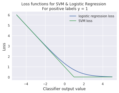

As in the previous homework, we’ll use sklearn. Read the manpage for SVM before starting the assignment. Most machine learning toolkits treat algorithms for the same type of task (in this case, classification) the same. You’ll find that training and testing an SVM is identical to training and testing the logistic regression classifier we generated in the previous homework. You are encouraged to reuse and, if helpful, simplify your code or the code found in the homework 5 solutions.

import numpy as np
import matplotlib.pyplot as plt
import sklearn.metrics
from sklearn.svm import SVC
from sklearn.linear_model import LogisticRegression

#data for assignment
training_data = np.loadtxt("homework_6_train.txt")
X_train = training_data[:,0:2] #selects columns 1 and 2, which are the x and y coords of the data
Y_train = training_data[:,2] #selections column 3, which is the 0 or 1 label of the data

test_data = np.loadtxt("homework_6_test.txt")
X_test = test_data[:,0:2]
Y_test = test_data[:,2]

#plotting each class seperately, not important for training the models
X_1 = []
X_2 = []
for row in range(X_train.shape[0]):
    if Y_train[row] == 0:
        X_1.append(X_train[row,:])
    else:
        X_2.append(X_train[row,:])
X_1 = np.asarray(X_1)
X_2 = np.asarray(X_2)

plt.scatter(X_1[:,0], X_1[:,1], label="Class 1")
plt.scatter(X_2[:,0], X_2[:,1], label="Class 2")
plt.legend()
plt.show()

Problem 1

Using a SVM on the training data set X_train and Y_train, train a classifier. Use the model object function settings I’ve provided below. Compute and print the training precision and recall. Additionally, compute the test precision and recall.

#insert your code here

svm_model_obj = SVC(gamma='auto', kernel='linear')

Problem 2

Train a logistic regression on the training data set X_train and Y_train. Compute the test precision and recall for the logistic regression classifier.

#insert your code here

Problem 3a

In this problem we’re going to look at the effect of an outlier on SVM and logistic regression. First, using the solution to the bonus problem in Homework 5, plot the data and the decision boundaries for both the SVM and logistic regression classifiers from problem 2.

#insert your code here

Problem 3b

Now we’ll add the outlier. With the new data sets X_train_outlier and Y_train_outlier, train a new SVM and logistic regression classifier. Plot the data and decision boundaries for both the newly trained SVM and logistic regression classifier. Note which classifier can handle the outlier and which can’t even when the data is clearly linearly seperable. This is in part due to the fact that logistic regression loss never goes to zero for correctly classified points. Conversely, if this outlier is in fact not representative of real data, consider how this will effect test performance.

X_train_outlier = np.vstack((X_train, np.array([5, -2.5])))  #adding the outlier
Y_train_outlier = np.concatenate((Y_train, np.array([1.0])))   #adding the label for the outlier

#insert your code here

Bonus 1

I’ve generated a data set that can only be seperated by a circluar boundary. This is the worst case scenario for a model that attempts to sepearte data with a straight line. But recall from our regression assignments: if we know the type of function we want to fit, we can pass the data through a kernel (in this problem we use the radial basis function (RBF)—a very powerful basis). Using the SVM model code you’ve written above and the data provided here, use the following model function settings to seperate the data and draw the decision boundary.

data_bonus = np.loadtxt("homework_6_bonus.txt")
X_b = data_bonus[:,0:2]
Y_b = data_bonus[:,2]

X_1 = []
X_2 = []
for row in range(X_b.shape[0]):
    if Y_b[row] == 0:
        X_1.append(X_b[row,:])
    else:
        X_2.append(X_b[row,:])
X_1 = np.asarray(X_1)
X_2 = np.asarray(X_2)

plt.gca().set_aspect('equal') 
plt.scatter(X_1[:,0], X_1[:,1], label="Class 1")
plt.scatter(X_2[:,0], X_2[:,1], label="Class 2")
plt.legend()
plt.show()

#insert your code here

svm_model_obj = SVC(gamma='auto', kernel='rbf')  #very important that the kernel setting is 'rbf'